Calculates number of instances for the comparison of multiple algorithms

Calculates either the number of instances, or the power(s) of the comparisons of multiple algorithms.

calc_instances(
  ncomparisons,
  d,
  ninstances = NULL,
  power = NULL,
  sig.level = 0.05,
  alternative.side = "two.sided",
  test = "t.test",
  power.target = "mean"
)

Arguments

ncomparisons: number of comparisons planned
d: minimally relevant effect size (MRES, expressed as a standardized effect size, i.e., "deviation from H0" / "standard deviation")
ninstances: the number of instances to be used in the experiment.
power: target power for the comparisons (see Details)
sig.level: desired family-wise significance level (alpha) for the experiment
alternative.side: type of alternative hypothesis to be performed ("two.sided" or "one.sided")
test: type of test to be used ("t.test", "wilcoxon" or "binomial")
power.target: which comparison should have the desired power? Accepts "mean", "median", or "worst.case" (this last one is equivalent to the Bonferroni correction).

Value

a list object containing the following items:

ninstances - number of instances
power - the power of the comparison
d - the effect size
sig.level - significance level
alternative.side - type of alternative hypothesis
test - type of test

Details

The main use of this routine uses the closed formula of the t-test to calculate the number of instances required for the comparison of pairs of algorithms, given a desired power and standardized effect size of interest. Significance levels of each comparison are adjusted using Holm's step-down correction (the default). The routine also takes into account whether the desired statistical power refers to the mean power (the default), median, or worst-case (which is equivalent to designing the experiment for the more widely-known Bonferroni correction). See the reference by Campelo and Wanner for details.

Sample Sizes for Nonparametric Methods

If the parameter test is set to either Wilcoxon or Binomial, this routine approximates the number of instances using the ARE of these tests in relation to the paired t.test, using the formulas (see reference by Campelo and Takahashi for details):

$$n.wilcox = n.ttest / 0.86 = 1.163 * n.ttest$$ $$n.binom = n.ttest / 0.637 = 1.570 * n.ttest$$

References

P. Mathews. Sample size calculations: Practical methods for engineers and scientists. Mathews Malnar and Bailey, 2010.
F. Campelo, F. Takahashi: Sample size estimation for power and accuracy in the experimental comparison of algorithms. Journal of Heuristics 25(2):305-338, 2019.
F. Campelo, E. Wanner: Sample size calculations for the experimental comparison of multiple algorithms on multiple problem instances. Submitted, Journal of Heuristics, 2019.

Author

Felipe Campelo (fcampelo@ufmg.br, f.campelo@aston.ac.uk)

Examples

# Calculate sample size for mean-case power
K      <- 10   # number of comparisons
alpha  <- 0.05 # significance level
power  <- 0.9  # desired power
d      <- 0.5  # MRES

out <- calc_instances(K, d,
                      power     = power,
                      sig.level = alpha)

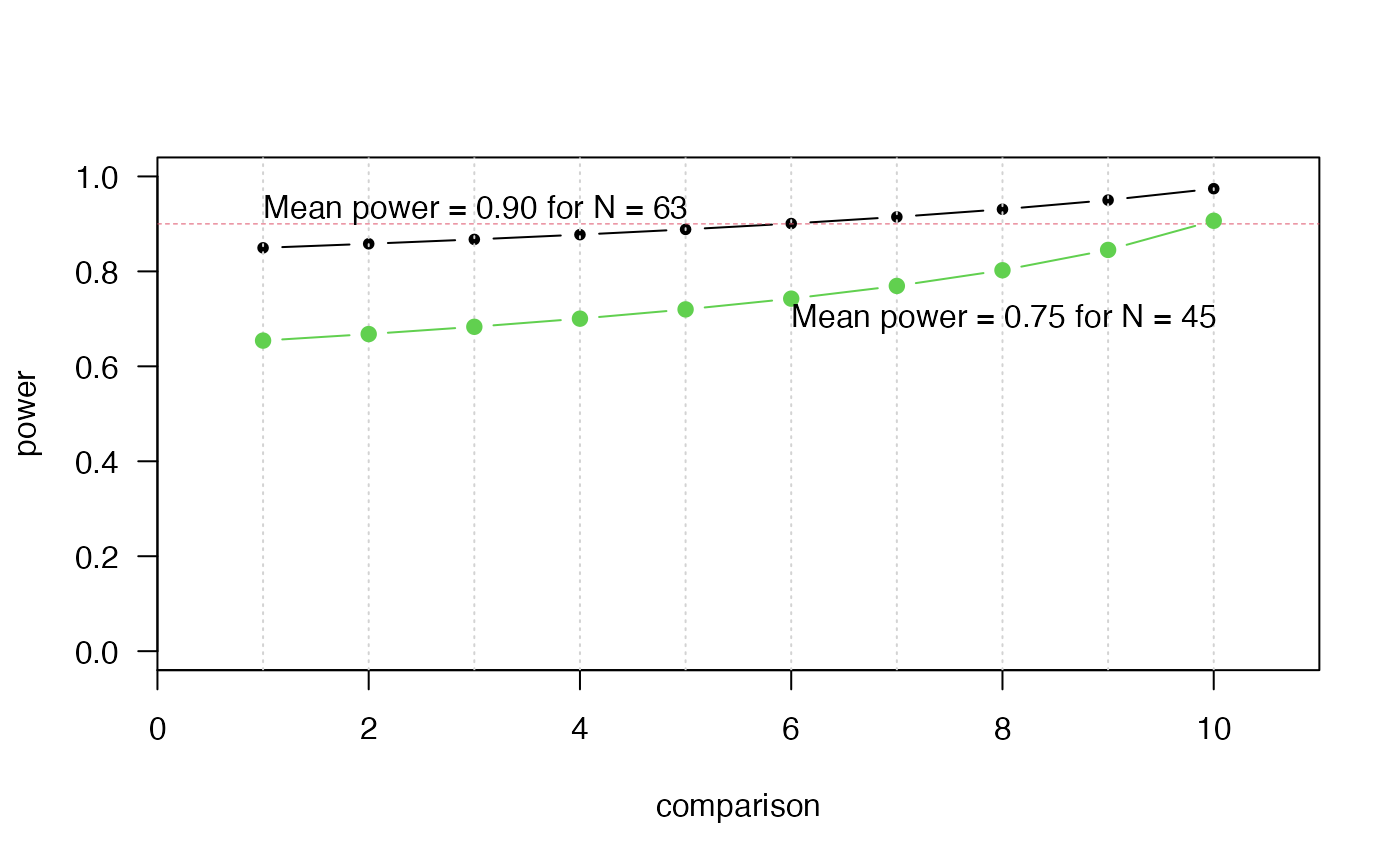
# Plot power of each comparison to detect differences of magnitude d
plot(1:K, out$power,
     type = "b", pch = 20, las = 1, ylim = c(0, 1), xlab = "comparison",
     ylab = "power", xaxs = "i", xlim = c(0, 11))
grid(11, NA)
points(c(0, K+1), c(power, power), type = "l", col = 2, lty = 2, lwd = .5)
text(1, 0.93, sprintf("Mean power = %2.2f for N = %d",
                     out$mean.power, out$ninstances), adj = 0)

# Check sample size if planning for Wilcoxon tests:
calc_instances(K, d,
               power     = power,
               sig.level = alpha,
               test = "wilcoxon")$ninstances
#> [1] 74


# Calculate power profile for predefined sample size
N <- 45
out2 <- calc_instances(K, d, ninstances = N, sig.level = alpha)

points(1:K, out2$power, type = "b", pch = 19, col = 3)
text(6, .7, sprintf("Mean power = %2.2f for N = %d",
                     out2$mean.power, out2$ninstances), adj = 0)


# Sample size for worst-case (Bonferroni) power of 0.8, using Wilcoxon
out3 <- calc_instances(K, d, power = 0.9, sig.level = alpha,
                       test = "wilcoxon", power.target = "worst.case")
out3$ninstances
#> [1] 83

# For median power:
out4 <- calc_instances(K, d, power = 0.9, sig.level = alpha,
                       test = "wilcoxon", power.target = "median")
out4$ninstances
#> [1] 76
out4$power
#>  [1] 0.8641640 0.8720871 0.8806398 0.8899412 0.9001496 0.9114838 0.9242583
#>  [8] 0.9389522 0.9563477 0.9777831